Topology of Representations
Persistent homology measures the shape of a set of points: its clusters, the loops they form, and the voids they enclose, and how long each lasts as the scale grows. Applied to a layer's activations, it asks questions the tools in Analyzing representations can't: does a layer arrange the days of the week on a circle, and does that circle survive noise and a random-network control?
pulsatrix builds this as a pipeline, one stage at a time:
PointCloud → distances → filtration → persistence diagram → numbers and plots
This page grows with each stage. So far it covers the point cloud, the distances, the diagrams (H0, then loops, voids and higher), how to compare diagrams, how to turn them into numbers, landmarks for large clouds, whether a feature is real, and comparing two representations' topology.
From activations to a point cloud
PointCloud gathers a layer's activations, batch by batch, into one set of points. Each point
remembers the sample and position it came from, so a loop found later can be traced back to the
inputs that form it.
#include "pulsatrix/tda/point_cloud.hpp"

PointCloud cloud({PointPooling::PerPosition});  // one point per token
model->set_hidden_state_hook([&](int64_t position, const Tensor& h) {
    if (position == 6) cloud.add(h);             // (1, tokens, width)
    return h;
});
for (const std::string& text : corpus) (void)model->forward(Encode(text));
// cloud.size() points of cloud.dimension() == width.
// cloud.origins()[i].sample is the text, .position the token.
How a sample becomes points is the one choice to make:
PointPooling |
Points per sample | Use it for |
|---|---|---|
Flatten (the default) |
One, every dimension after the batch flattened | An MLP layer, a classifier's logits |
PerPosition |
One per token or pixel | The geometry of token representations |
Mean, Max |
One, pooled over the positions | A summary of an encoder's whole input |
Last |
One, the last position | A causal language model's summary of the whole input |
- The feature axis. For every pooling but
Flatten,PointCloudOptions::feature_axissays which axis holds the features. The default, the last axis, suits a sequence model's(batch, tokens, width). Use1for a convolution's(batch, channels, height, width); its pixels then become the positions, in row-major order. - Batches of different lengths. The first batch fixes the points' dimension. Later batches can have any number of positions, so texts of different lengths go in one at a time. Sample numbers keep counting across batches.
- Snapshots.
cloud.add(snapshot, node)adds one node of anExplainerContextsnapshot.MakePointCloud(snapshots, node)builds a cloud from several. - Checks. A batch with a NaN or infinity, or of the wrong dimension, throws and adds nothing.
Meansums in double precision.
cloud.ToTensor(&backend) gives the points as an (n, dimension) tensor for the stages that
follow.
Distances, with an error bar
Persistent homology sees the points only through their pairwise distances. PairwiseDistances()
computes them as |x|² + |y|² − 2 x·y, with the dot products from one GEMM on the cloud's backend
(CPU, HIP or CUDA):
#include "pulsatrix/tda/distance_matrix.hpp"

const DistanceMatrix d = PairwiseDistances(cloud, &backend);
// d.values: the n (n − 1) / 2 distances, in scipy's pdist order; d.at(i, j) reads one.
// d.error_bound: every stored distance is within this of the exact one.
Why the error bound. In float32 that formula cancels for points close together, relative to
their distance from the origin. The result can be wrong in every digit, and since persistent
homology is all about small distances (when do two points join?), that matters. So every
DistanceMatrix carries a certified bound: |stored − exact| ≤ error_bound for every pair.
- It's rigorous. It comes from the standard error analysis of a float32 dot product (at most γ_d ‖x‖ ‖y‖, whatever order the GEMM sums in), plus the double-precision steps and the final rounding. It assumes the GEMM accumulates in float32, not TF32 or bf16.
- It carries through. Persistence diagrams are stable: a diagram computed from these
distances is within
error_bound, in bottleneck distance, of the exact one. Later stages add their own errors to it. - When it's large, center. Points sharing a large offset, as in an anisotropic layer, make
the bound large.
DistanceOptions::centersubtracts the mean first, which leaves the distances unchanged. In the tests, points spread by 0.01 per coordinate, sitting 1,000 from the origin, get a bound bigger than a tenth of their distances. Centered, it shrinks over a hundredfold, to under a thousandth. - Or compute exactly.
DistanceMethod::Exactsums squared differences in double on the host. Its bound is the float32 rounding of the result, but it costs n² × d on the CPU.
Other options:
normalizescales every point to unit length first. The distance is then √(2 − 2 cos), a metric that orders pairs as cosine similarity does.block_rowssets how many rows each GEMM computes. The device holds the points and one block at a time; by default a block has at most 2²⁴ entries.
Storing n (n − 1) / 2 float32 values takes 50 MB for 5,000 points. Persistent homology above H0 can't use many more points than that anyway; landmarks choose which ones to keep.
Clusters across scales (H0)
Grow a ball around every point. At scale 0 each point is its own component. As the scale grows, two components merge when the shortest edge between them appears, until one is left. H0 persistence records those merges: one pair (born at 0, dies at the merge scale) per merge, and one pair that never dies.
That is single-linkage clustering, and the merge scales are the edge lengths of a minimum
spanning tree. ComputeH0() finds the tree exactly with Prim's algorithm, in O(n²) time:
#include "pulsatrix/tda/h0.hpp"

const H0Result h0 = ComputeH0(PairwiseDistances(cloud, &backend));
// h0.diagram.pairs: (0, merge scale) per merge, then (0, ∞). h0.diagram.error_bound is the
// distances' bound: the diagram is within it of the exact one, in bottleneck distance.
// h0.edges: the tree's n − 1 edges, shortest first; edge k is the k-th merge.
const std::vector<int64_t> clusters = SingleLinkageClusters(h0.edges, cloud.size(), /*threshold=*/0.5);
- Long-lived pairs are clusters. A pair that dies late means a group that stays apart from
the rest over a wide range of scales.
SingleLinkageClusters()cuts the tree at a scale and labels the groups. Each edge's endpoints, throughcloud.origins(), name the inputs a merge joins. - Duplicate points give zero-length edges. They stay in
edgesbut not in the diagram, which leaves out zero-persistence pairs as Ripser does. - Ties in length break by the lower point index, so the tree is the same on every platform. Its lengths, which are all the diagram uses, are the same for every minimum tree.
H0 alone says little. It is a function of the minimum spanning tree, so it sees roughly what nearest-neighbor distances see. Many recent papers on the topology of language models use only H0. Before trusting such a result, check it against plain nearest-neighbor statistics. Loops and voids (H1, H2) are where persistent homology sees something new.
Loops and voids (H1, H2 and up)
ComputeRipsPersistence() computes the diagrams of the Vietoris–Rips filtration in every
dimension up to max_dimension. A simplex joins the complex at its diameter, and loops (H1)
and voids (H2) form and fill in as the scale grows:
#include "pulsatrix/tda/rips_persistence.hpp"

RipsOptions options;
options.max_dimension = 2;   // H0, H1 and H2
const RipsResult r = ComputeRipsPersistence(PairwiseDistances(cloud, &backend), options);
for (const RipsFeature& loop : r.features[1]) {
    // loop.pair.birth, loop.pair.death; r.diagrams[1] has the same pairs.
    // loop.birth_edge, loop.death_edge: the edges whose lengths are the birth and the death.
}
- Where a feature comes from. Each feature names its critical edges. The birth edge is the
longest edge of the simplex that creates the feature; the death edge is the longest edge of
the one that fills it in. Their endpoints, through
cloud.origins(), are inputs. - Representative cocycles. With
RipsOptions::cocycles, each feature in H1 and up comes with a cocycle: a value on edges (for H1) whose coboundary vanishes on every triangle present before the death. A loop's cocycle is nonzero summed around the loop. Circular coordinates, which place points on the loop, are built from it. - Coefficients.
coefficientis the prime p of the field Z/p, 2 by default. Diagrams over different primes differ only for spaces with torsion, such as the projective plane. Circular coordinates need a prime above 2, to lift the cocycle to the integers. - The threshold. By default it is the enclosing radius, the smallest over points of the
distance to the farthest one. There the complex is a cone, so every loop and void has died
and nothing is cut short. With a lower
threshold, features still alive at it are reported as essential (death ∞).
How it is computed. It follows the algorithm of Bauer's Ripser (2021), written for pulsatrix rather than vendored:
- persistent cohomology, which pairs the same intervals as homology;
- simplices named by their index in the combinatorial number system, with coboundaries enumerated on demand rather than stored;
- clearing, and zero-persistence apparent pairs, which are settled without any reduction.
On a CPU (Release build, points in 3 dimensions) it takes:
| Points | Dimensions | Time | Memory |
|---|---|---|---|
| 1,000 | H0, H1 | 0.25 s | |
| 2,000 | H0, H1 | 1.2 s | |
| 300 | H0 to H2 | 0.5 s | |
| 600 | H0 to H2 | 4.1 s | 125 MB peak for the whole run |
Cost grows quickly with the number of points and the dimension. Above a few thousand points for H1, or about a thousand for H2, choose landmarks first.
How it is checked. Nothing here relies on another library's output:
- A theorem. Evenly spaced points on a circle have a known Rips complex at every scale (Adamaszek and Adams, 2017). For 12 points: one loop from the side length to the chord of 4 steps, then exactly three voids from there to the chord of 5 steps.
- Betti numbers from scratch. For every subset of 7 random points, at every scale, the ranks of the boundary matrices over Z/2 and Z/3 give the Betti numbers. The pairs alive at that scale must match them in every dimension.
- The Euler characteristic. On 8 random points it matches at every scale.
- The cocycle condition, and the winding of a circle's cocycle.
- H0 matches the minimum spanning tree.
Comparing diagrams
Two diagrams, say of the same layer in two models, two seeds, or before and after fine-tuning, are compared by matching their points. Each point goes either to a point of the other diagram or to the diagonal, where a feature of zero persistence would sit:
#include "pulsatrix/tda/diagram_distance.hpp"

const Certified<double> d = BottleneckDistance(base.diagrams[1], tuned.diagrams[1]);
// d.value: the largest move in the best matching.
// d.bound(): the exact diagrams' distance is within this of d.value; d.terms itemize it.
const double w2 = WassersteinDistance(base.diagrams[1], tuned.diagrams[1], /*order=*/2);
- Bottleneck distance is the smallest possible largest move. It is the distance the stability theorem uses (Chazal, de Silva and Oudot, 2014): if two clouds' distance matrices differ by at most e, their Rips diagrams are within e. The tests check this on random clouds and perturbations, in H0 and H1, and the bound comes close to tight.
- Wasserstein distance W_q is the q-th root of the smallest sum of q-th powers of the moves. It counts every feature, where the bottleneck counts only the worst one. As q grows it approaches the bottleneck.
- Moves are measured in the L∞ norm, as in the stability theorem, so a point (b, d) is (d − b) / 2 from the diagonal. Essential features are matched to each other by birth. If two diagrams have different numbers of them, the distance is infinite.
Certified values. Certified<T> holds a value and the error terms behind it, each with its
source. A bottleneck distance carries both diagrams' error_bounds: by the triangle inequality,
the distance between the exact diagrams is within their sum. So a difference between two
layers is real only if it exceeds d.bound().
The Wasserstein distance isn't certified. An error of e in every distance can move it by up to e times the q-th root of the number of points, so a single bound would mean little.
Both are exact. The bottleneck distance uses a binary search over candidate values, each tested by a Hopcroft–Karp matching, and is comfortable up to a few hundred points per diagram. The Wasserstein distance uses the Hungarian algorithm, which takes (n₁ + n₂)³ time, so up to about a thousand points in all. Both match brute force over every matching on small diagrams.
Diagrams as numbers
A probe, a t-test or a plot needs a fixed-size vector, not a set of points. Four standard
vectorizations are in tda/vectorization.hpp:
#include "pulsatrix/tda/vectorization.hpp"

const std::vector<double> grid = LinearGrid(0.0, r.threshold, 100);
const std::vector<int64_t> betti = BettiCurve(r.diagrams[1], grid);           // loops alive at each t
const Certified<PersistenceLandscape> l = ComputePersistenceLandscape(r.diagrams[1], grid, /*layers=*/5);
const PersistenceImage image = ComputePersistenceImage(r.diagrams[1], image_options);
const double entropy = PersistentEntropy(r.diagrams[1]);
| Vectorization | What it is | Stable? |
|---|---|---|
| Betti curve | How many features are alive at each scale | No: a point crossing a grid value changes it by 1 |
| Persistence landscape (Bubenik, 2015) | λ_k(t), the k-th largest "tent" min(t − b, d − t) at each t | Yes: within the bottleneck distance, at every t. Certified. |
| Persistence image (Adams et al., 2017) | Points at (birth, persistence), weighted by persistence, blurred by a Gaussian, integrated over pixels | Under the 1-Wasserstein distance, not the bottleneck |
| Persistent entropy | The Shannon entropy of the lifetimes, in nats | Not in general |
- Prefer landscapes when the result has to hold up. They are the only one of the four that
inherits the stability theorem.
ComputePersistenceLandscapereturns aCertifiedvalue: the exact diagram's landscapes are withinbound()of these at every grid point. - Fix the image's ranges when comparing. By default a persistence image takes its birth and
persistence ranges from its own diagram. Images of two diagrams are comparable only with
birth_max,persistence_maxandsigmaset the same for both. - Essential features are left out of everything except the Betti curve, where they count
from their birth on. Report how many there are (
essential_count()) alongside.
Landmarks for large clouds
A layer's activations over a dataset can be 100,000 points, far more than H1 or H2 can handle.
FarthestPointLandmarks() picks a subset that covers the whole cloud. Each landmark is chosen
greedily as the point farthest from those already picked:
#include "pulsatrix/tda/landmarks.hpp"

LandmarkOptions options;
options.count = 1000;            // or options.radius: stop once every point is that close
const Landmarks l = FarthestPointLandmarks(cloud, &backend, options);
const Tensor subset = LandmarkPoints(cloud.ToTensor(&backend), l);
const RipsResult r = ComputeRipsPersistence(PairwiseDistances(subset), rips_options);
const PersistenceDiagram loops = WithSubsamplingBound(r.diagrams[1], l);
// loops.error_bound now bounds the bottleneck distance to the diagram of *all* the points.
- The certified bound. Every point is within the covering radius ε of a landmark, so the
landmarks' Rips diagrams are within 2ε of the whole cloud's in bottleneck distance.
l.covering_radiusis aCertifiedvalue whose term is the float32 error of the distances behind it.WithSubsamplingBound()adds 2 × (ε + that error) to a diagram's own bound. A feature of the landmarks with persistence well above twice that is a feature of the cloud. - Choosing the count.
l.insertion_radii[k]is the covering radius just before landmark k was added. It only decreases; plot it and stop where it flattens. Greedy selection is within a factor of 2 of the best possible covering radius for the same count (Gonzalez, 1985). The tests check this against brute force on small clouds. - Cost. Each landmark costs one GEMM of all the points against it, on the cloud's backend, so k landmarks take O(n k d). The n × n distance matrix is never formed.
- Ties go to the lowest index.
options.firstsets the first landmark.options.centershrinks the float32 error when the points share a large offset, as it does for distances. - Where each point went.
l.nearest[i]andl.distance_to_nearest[i]give each point's landmark. Use them to carry labels or inputs over from the landmarks back to the whole cloud.
In the tests, 50 landmarks of a noisy circle of 300 points give an H1 diagram within its certified bound of the full diagram, and the circle's loop persists more than four times longer than the bound.
Is a feature real?
A diagram of pure noise is full of short-lived loops, and some always live longer than the rest.
Before reporting a loop, test it. tda/significance.hpp has three tests, each answering a
slightly different question.
The universal null: one diagram, a p-value per feature. Bobrowski and Skraba (2023) found that the death/birth ratios of noise follow one distribution, whatever the noise came from, once normalized: ℓ = log log(death / birth) − L̄ − γ, where L̄ is the diagram's mean of log log(death / birth) and γ is Euler's constant. Under the null, ℓ follows a left-skewed Gumbel distribution, so a feature's p-value is exp(−e^ℓ). Bonferroni's correction then splits α over the features.
#include "pulsatrix/tda/significance.hpp"

const UniversalNullResult u = UniversalNullTest(r.diagrams[1], /*alpha=*/0.05);
for (const FeatureSignificance& f : u.features) {
    if (f.significant) { /* r.features[1][f.index] is a real loop */ }
}
- It's a conjecture, supported by the authors' experiments on many distributions and real data, not a theorem. The constants are theirs for Rips filtrations (A = 1).
- It needs a mostly-noise diagram. L̄ comes from the diagram itself, so use diagrams with hundreds of features or more. Point sets spaced too evenly, such as lattices, don't follow it.
- In the tests, the p-values of the loops of uniform noise are calibrated (about a tenth fall below 0.1, and half below 0.5), and Bonferroni flags at most one of their 300-odd loops. A ring with clutter around it is flagged; the same ring with uniform points inside it isn't, since those points fill the loop in at once.
The bootstrap band: how far the diagram moves under resampling. BootstrapBand() resamples
the points with replacement, computes each resample's diagram, and takes the 1 − α quantile c
of their bottleneck distances to the original (Fasy et al., 2014). Features with persistence
above 2c lie outside the band. Resamples reuse the distance matrix, so nothing is recomputed,
but each one is a full Rips computation. Fasy et al. prove coverage for distance-function
filtrations; for Rips diagrams the band is the standard heuristic.
Baselines: is this more structure than a cloud with nothing in it? Compute a statistic, such
as MaxPersistence() of H1, on the data and on clouds with no structure, then take
BaselinePValue(), the rank p-value:
GaussianBaseline(points, count, seed)draws a Gaussian cloud with the same mean and covariance (one GEMM, and the covariance's rank is kept, so a cloud in a plane gives a baseline in the same plane);- for a random-network baseline, collect the same layer's activations from a
NullModelBaselinecopy of the model.
With m baselines the smallest p-value is 1 / (m + 1): use 19 for p = 0.05, 99 for 0.01.
Use more than one. The universal null is cheapest, and the bootstrap needs no conjecture. The random-network baseline is the one that asks whether the structure was learned.
For all of them on a real model, see the recipe Is the shape real?. It tests the calendar circle in SmolLM2-135M and Llama-3.2-1B, and one of its lessons is a caution: on points that come in tight clusters, the largest death/birth ratio can pick loops inside the clusters rather than the ring through them.
Seeing the result
viz/topology_documents.hpp saves diagrams as a pulsatrix.persistence_diagram.v1 document,
with each dimension's certified error bound and any test results. viz/topology_views.hpp draws
the document three ways:
RenderPersistenceDiagramSvg: birth against death. A gray band along the diagonal covers persistence up to twice the error bound, which errors in the distances alone could explain. Features that never die sit on a dashed ∞ line.RenderBarcodeSvg: one bar per feature, longest first, with ±error-bound whiskers.RenderBettiCurveSvg: how many features are alive at each scale. The error bound doesn't cover it, since short features can come and go; the figure says so.
With a test attached, significant features are drawn filled (diagram) or solid (barcode), and the rest hollow or faint:
#include "pulsatrix/viz/topology_views.hpp"

PersistenceDiagramDocument doc = ToPersistenceDiagramDocument(r, "Layer 12, weekday tokens");
AttachSignificance(doc, 1, UniversalNullTest(r.diagrams[1]));   // p-values on H1
std::ofstream("diagram.svg") << RenderPersistenceDiagramSvg(doc);
std::ofstream("doc.json") << ToJson(doc);   // later: pulsatrix_svg doc.json --view barcode
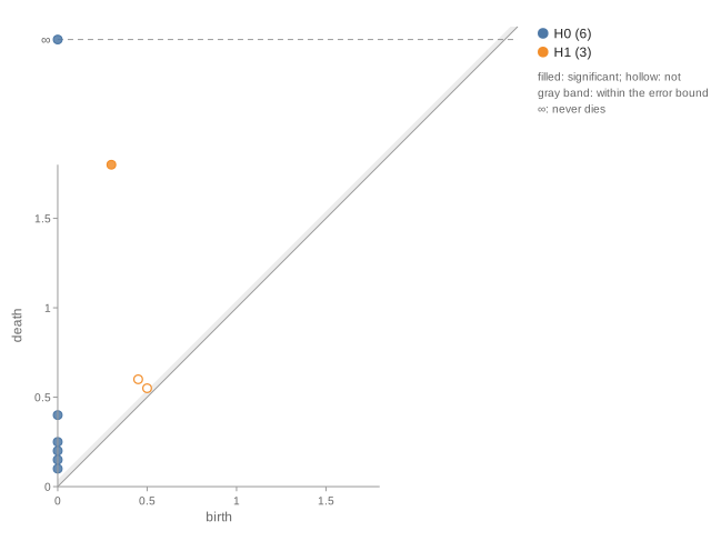
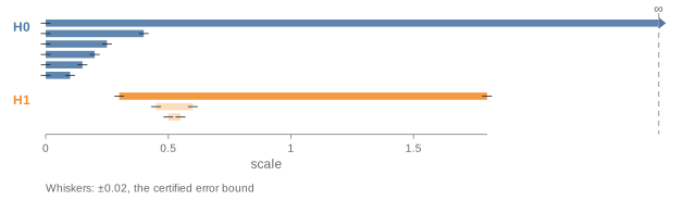
On the command line: pulsatrix_svg doc.json --view diagram|barcode|betti [--dims 1]. There is
no HTML view yet.
Comparing two representations' topology (RTD)
CKA compares two representations' whole geometry at once. When most of the variance is in a few large distances, it can call two layers alike although one splits a cluster that the other keeps whole. Representation Topology Divergence (Barannikov, Trofimov et al., 2022) compares the clusters and loops at every scale:
#include "pulsatrix/tda/rtd.hpp"

const RtdResult r = Rtd(layer_a, layer_b);   // rows: the same inputs, in the same order
// r.rtd: 0 for the same topology; larger means more clusters and loops differ, and by more.

const RepresentationComparison c = CompareRepresentations(layer_a, layer_b);
// c.cka, c.mutual_knn, c.rtd.rtd: three views side by side.
- How it works. Each representation's distances are divided by their 0.9 quantile, so
scale doesn't count. A Vietoris–Rips filtration on two copies of the inputs then mixes the two
sets of distances. Its H1 barcode, the R-Cross-Barcode, holds a bar for each cluster that
merges at one scale in one representation and at another scale in the other. RTD is the
total length of those bars, averaged over both directions and over random batches of 500
inputs (
RtdOptions, as in the paper's Algorithm 2). - What it guarantees. The cross-barcode of identical representations is empty. Against distances that are all 0, it is the ordinary barcode one dimension down (the paper's Theorem 2.1). The tests check both exactly, and that rotation and scale leave RTD near 0.
- In the tests, two clusters 40 apart, each then split in two, keep CKA above 0.9, while RTD rises almost fivefold over a jittered copy. Mutual-kNN alignment drops too: it sees the neighbors change.
CrossBarcode(w, w~, dimension)gives the barcode itself, for your own distances (not normalized), to see which clusters differ.- Cost. Each batch is a Rips computation on twice the batch size.
Full API reference: Doxygen: Topological Data Analysis