Visualization

Use this section to see your model's explanations and training progress as charts instead of numbers. It provides native C++ charts, dashboards, and live views built on Dear ImGui and ImPlot (immediate-mode GUI and plotting libraries).

The explainers, LRP rules, and interpretability tools elsewhere in pulsatrix return plain data (Attribution, CircuitGraph, ActivationSnapshot) and never draw anything. This layer is optional and sits on top of that data. pulsatrix_core never depends on it, the same way core does not depend on the Python bindings (pulsatrix_py).

What's inside

Data transforms (viz/plot_data.hpp, viz/colormap.hpp). These are plain functions with no ImGui or ImPlot code. They are always compiled into pulsatrix_core and are unit-tested:

• ToFeatureImportanceBars / ToWaterfallSteps / ToWaterfallBars: turn an Attribution into sorted bars, or into a waterfall from the baseline to the prediction.
• CircuitNodeDisplayLabel: a readable label for a CircuitGraph node.
• ToSaliencyHeatmap / ComputeHeatmapColorScale: turn an Attribution into a 2D grid and choose its color scale. The scale is symmetric around zero when any value is negative, and [0, max] otherwise.
• ToBeeswarmPoints: spread one feature's values across many Attributions into non-overlapping points. The jitter is deterministic.
• ToFieldHistogramBins: bin a Dataset field's values into an equal-width histogram.
• ToRgbImageBuffer: convert an image Tensor into bytes ready for a GPU texture.
• ViridisColormap / DivergingColormap: colorblind-safe colormaps for unsigned and signed values.

Metrics sink (viz/implot_metrics_sink.hpp). ImPlotMetricsSink is a MetricsSink that stores every logged scalar and histogram as a per-tag series. Its logging methods (log_scalar(), log_histogram()) are compiled into pulsatrix_core and need no flag. Only Draw() needs pulsatrix_viz. To write your own sink, see Adding a new metrics sink.

Chart widgets (only with PULSATRIX_ENABLE_VIZ=ON). Each one is a thin ImGui/ImPlot drawing call over the data transforms:

Widget	Shows
AttributionBarChart	Top features of one attribution, as bars
AttributionWaterfallChart	How features move the output from the baseline to the prediction
AttributionBeeswarmView	One feature's attribution across many inputs
SaliencyHeatmapView	An attribution laid over an image
CircuitGraphView	A CircuitGraph's per-node ablation effect
ConfidenceMeter	A confidence value as a labeled bar
ExplanationScoreCard	One panel: prediction, top features, confidence, and trust checks (ComputeConservation, ComputeAttributionStability)
DatasetStatisticsView	Per-field histograms of a dataset
ImageGridView	A grid of image thumbnails with captions
TrainingDashboard, ImPlotMetricsSink::Draw()	Live training curves

Infrastructure. VizWindow (viz/window.hpp) owns the window, the OpenGL context, and the ImGui/ImPlot setup. You write a per-frame draw callback and call window.run(...). TextureCache uploads images to the GPU once and reuses them across frames.

Full API reference: Doxygen: Visualization

Building with visualization enabled

Prerequisites

The default build has no GUI dependencies. -DPULSATRIX_ENABLE_VIZ=ON adds these:

• Network access at configure time. CMake downloads GLFW 3.4, Dear ImGui v1.90.9, and ImPlot v0.16 with FetchContent.
• OpenGL development files. CMake runs find_package(OpenGL REQUIRED). On Debian/Ubuntu, install libgl1-mesa-dev.
• GLFW's build dependencies on Linux. GLFW 3.4 builds X11 and Wayland support by default. On Debian/Ubuntu, install libx11-dev libxrandr-dev libxinerama-dev libxcursor-dev libxi-dev for X11, and libwayland-dev libxkbcommon-dev wayland-protocols for Wayland. To skip Wayland, add -DGLFW_BUILD_WAYLAND=OFF.
• A display and a GPU driver to run anything that links pulsatrix_viz. That is why the option defaults to OFF and CI builds without it.

Build

cmake -S . -B build -DPULSATRIX_ENABLE_VIZ=ON
cmake --build build --target training_dashboard_demo --config Release

Link your own executable against pulsatrix_viz. It brings in pulsatrix_core, imgui, and implot, including their include directories:

add_executable(my_viz_app my_viz_app.cpp)
target_link_libraries(my_viz_app PRIVATE pulsatrix_viz)

The data transforms and ImPlotMetricsSink's logging methods need no flag. They are always part of pulsatrix_core.

Demo apps

Target	What it shows
training_dashboard_demo	Live loss curves while an XOR network trains
explanation_dashboard_demo	Bar chart, waterfall, saliency heatmap, circuit graph, and score card for a small XOR network
dataset_preview_demo	DatasetStatisticsView and ImageGridView on small synthetic datasets
live_inference_demo	An ExplanationScoreCard that updates as it cycles through XOR inputs
mnist_viz_gallery	Every widget on MNIST digits (see below)

How to implement

A live training dashboard

#include <imgui.h>

#include "pulsatrix/adam_optimizer.hpp"
#include "pulsatrix/cpu_backend.hpp"
#include "pulsatrix/viz/training_dashboard.hpp"
#include "pulsatrix/viz/window.hpp"
#include "pulsatrix/xor_training_example.hpp"

using namespace pulsatrix;

CPUBackend backend;
XorNetwork net(&backend);
AdamOptimizer optimizer(0.05f, &backend);
ImPlotMetricsSink sink;  // a MetricsSink that buffers logged values for plotting

// The four XOR examples, as (1, 2) inputs and (1, 1) targets.
const float xs[4][2] = {{0, 0}, {0, 1}, {1, 0}, {1, 1}};
const float ys[4] = {0, 1, 1, 0};
int step = 0;

VizWindow window("Training Dashboard", 1000, 700);
window.run([&]() {
    for (int i = 0; i < 4 && step < 4000; ++i, ++step) {   // a few training steps per frame
        Tensor input(Shape({1, 2}), &backend, {xs[step % 4][0], xs[step % 4][1]});
        Tensor target(Shape({1, 1}), &backend, {ys[step % 4]});
        net.train_step(input, target, optimizer, sink, step);  // logs the loss to sink
    }
    ImGui::Begin("Training Dashboard");
    TrainingDashboard::Draw(sink);
    ImGui::End();
});

Full source: examples/viz/training_dashboard_demo.cpp.

What's happening: XorNetwork::train_step() and MnistConvNet::train_step() take a MetricsSink&. Passing an ImPlotMetricsSink adds plotting with no change to the training code. Each frame, TrainingDashboard::Draw() reads the sink's per-tag series. It draws a one-line summary per tag (last, min, max, current step) and a small line chart for each tag.

Logging and drawing are separate methods. The logging half works, and is unit-tested, even with PULSATRIX_ENABLE_VIZ=OFF. Only Draw() needs the GUI stack.

Recipe: Training dashboard.

MNIST gallery

mnist_viz_gallery runs every widget on this page against MNIST test digits:

python3 tools/fetch_mnist.py              # once: data/MNIST/raw/ (gitignored)
cmake -S . -B build-viz -DPULSATRIX_ENABLE_VIZ=ON -DCMAKE_BUILD_TYPE=Release
cmake --build build-viz --target mnist_viz_gallery -j
./build-viz/mnist_viz_gallery                          # interactive
./build-viz/mnist_viz_gallery --screenshot out/        # one PNG per page, then exit

Run it from the repository root, or pass --data DIR (default data/MNIST/raw).

Option	Meaning	Default
--epochs N	Training epochs	1
--train N	Training digits (about 25 s per epoch on one CPU core at the default)	60000
--images N	Test digits explained with every method. If none is misclassified, the first misclassified test digit is added.	4
--eval N	Held-out digits for the accuracy curve	2000
--beeswarm N	Digits behind each beeswarm	200
--screenshot DIR	Save one PNG per page to DIR, then exit	off

Page	Widgets	What it shows
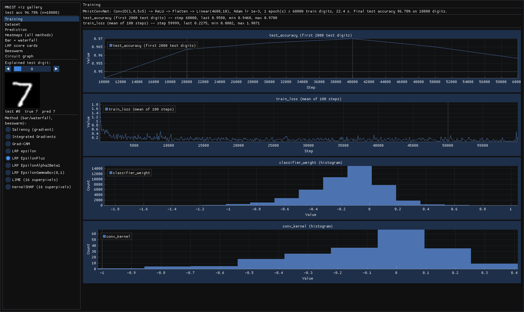
Training	ImPlotMetricsSink, TrainingDashboard	MnistConvNet (Conv2D(1,8,5x5) -> ReLU -> Flatten -> Linear) training live: 100-step mean loss, held-out accuracy, final conv-kernel and classifier-weight histograms
Dataset	DatasetStatisticsView, ImageGridView, TextureCache	Pixel and label histograms of the first 1000 test digits; 32 test digits captioned with true and predicted label
Prediction	ConfidenceMeter	10-class softmax of the selected digit
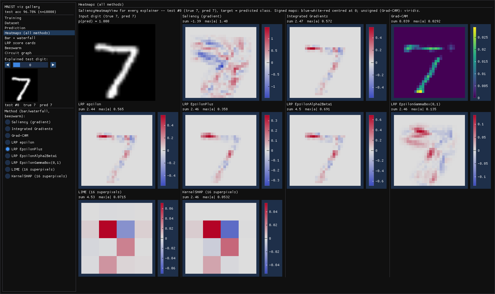
Heatmaps	SaliencyHeatmapView	Saliency, IG, Grad-CAM, LRP epsilon / EpsilonPlus / EpsilonAlpha2Beta1 / EpsilonGammaBox(0,1), LIME, KernelSHAP side by side
Bar + waterfall	AttributionBarChart, AttributionWaterfallChart	Top-12 features of the selected method, starting from its reference value (black-image logit for IG/SHAP, 0 otherwise)
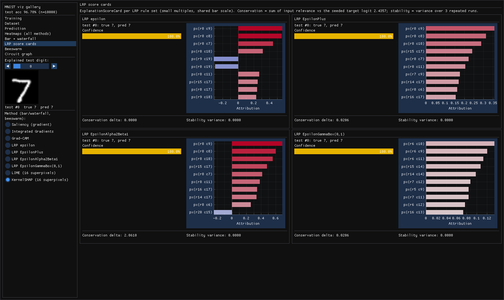
LRP score cards	ExplanationScoreCard	One card per LRP rule set, on a shared scale: confidence, top relevance, conservation delta, stability over repeated runs
Beeswarm	AttributionBeeswarmView	The 4 pixels with the highest mean |attribution| across 200 test digits, per gradient/LRP method
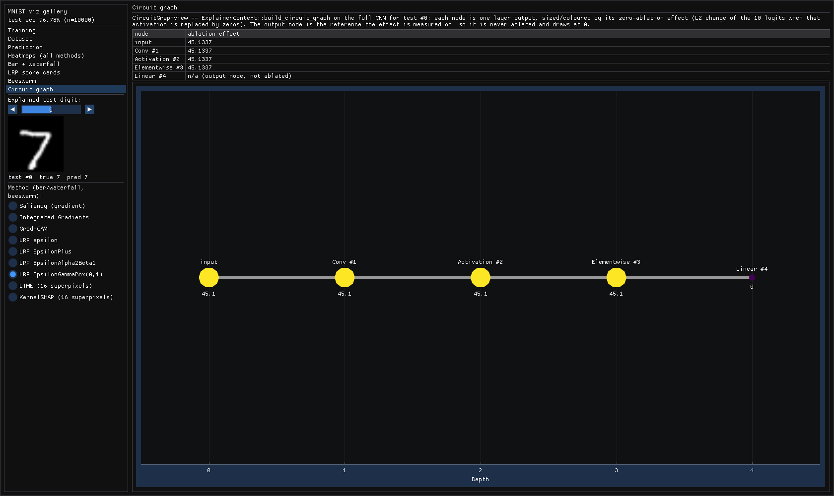
Circuit graph	CircuitGraphView	ExplainerContext::build_circuit_graph on the CNN: per-layer zero-ablation effect

For what the LRP rule names mean, see LRP.

Explainer settings

Method	Setting
Integrated Gradients	128 steps from a black baseline
Grad-CAM	The 24x24 map is zero-padded by 2 px onto the 28x28 grid, so each cell sits at the center of its 5x5 receptive field
KernelSHAP	16 superpixels (a 4x4 grid of 7x7 patches); all 2^16 coalitions enumerated exactly; an absent patch is black
LIME	The same 16 superpixels; 2000 samples; sigma 0.5

Why LIME uses superpixels

This library's LIME sets its locality kernel width equal to the perturbation sigma. On all 784 pixels, every sample weight underflows to zero, so pixel-level LIME is not meaningful here.

The gallery prints the test accuracy to stdout. For each explainer it also prints the attribution sum, the max |attribution|, and the IG-completeness, SHAP-efficiency, or LRP-conservation check.

Signed attributions use the blue-white-red diverging map, centered on zero. Unsigned ones (Grad-CAM) use Viridis. SaliencyHeatmapView picks the map via ComputeHeatmapColorScale.

Screenshots

Captured with --screenshot on a model trained for one epoch (96.78% test accuracy), test digit #0 (a 7):

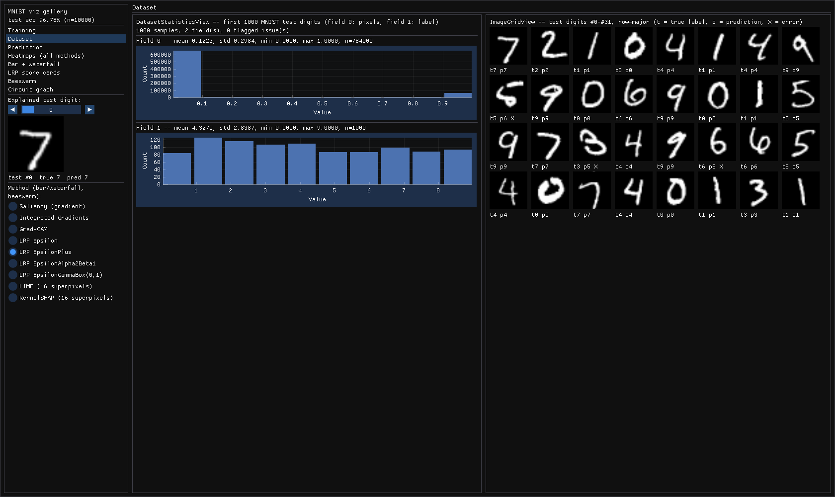Training: live loss, held-out accuracy, weight histograms	Dataset: pixel/label histograms, captioned test digits (X = misclassified)
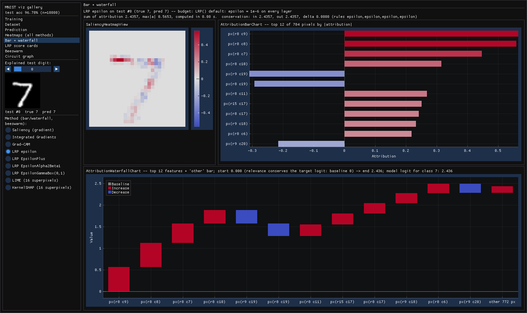Heatmaps: all nine explainers side by side	LRP epsilon: heatmap, top-12 bars, waterfall to the 2.436 logit
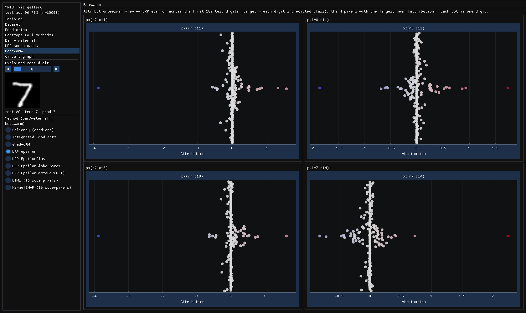Score cards: one per LRP rule set, conservation and stability	Beeswarm: top-4 pixels across 200 test digits
Circuit graph: per-layer zero-ablation effect (the output node is the reference, not ablated)

Recipes

• Training dashboard